
Soil Resistivity — Wenner Apparent Resistivity
What this calculation gives you
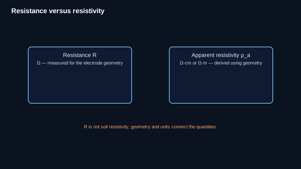
Convert the measured resistance and equal electrode spacing from a valid four-pin Wenner test into apparent soil resistivity. The field resistance reading is an input; it is not itself soil resistivity.
Governing equation(s)
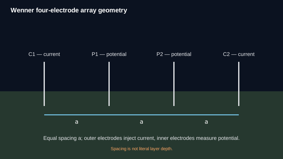
For four collinear, equally spaced pins with outer current electrodes and inner potential electrodes:
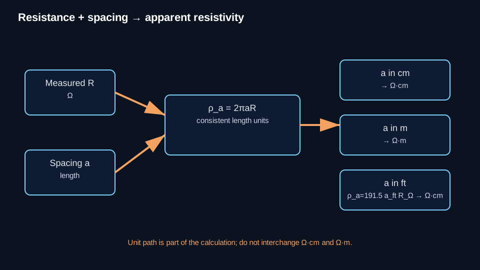
ρa = 2πaR
If potential and current are measured separately: R = V/I, so ρa = 2πa(V/I).
For spacing in feet and output in Ω·cm: ρa(Ω·cm) = 191.5 × aft × RΩ.
Variables
| Symbol | Meaning |
|---|---|
| ρa | apparent soil resistivity |
| a | equal Wenner pin spacing; directly measured geometry, not literal depth |
| R | measured electrical resistance |
| V | measured potential used to determine resistance where applicable |
| I | measured current used to determine resistance where applicable |
Units
- If
ais in centimetres andRis in ohms,ρais inΩ·cm. - If
ais in metres andRis in ohms,ρais inΩ·m. - If spacing is in feet and output is
Ω·cm, use the controlled191.5form. 1 Ω·m = 100 Ω·cm.
The formula constant never removes the need to identify the input length unit and output resistivity unit.
Conditions and assumptions
- Four collinear, equally spaced electrodes are used, with outer current and inner potential electrodes.
- The basic
2πaRrelationship uses the authorized equal-spacing Wenner geometry and standard shallow-electrode approximation. - The input resistance comes from a valid field measurement; this calculation does not validate the field test.
- Nearby parallel metallic structures, poor connections/contact, inadequate sensitivity, or electrode polarization can invalidate or distort measurements.
- The complete field procedure remains a conditional Method and is not published by this Calculation.
Worked calculation
Given: equal pin spacing a = 5 ft; measured resistance R = 10 Ω.
ρa(Ω·cm) = 191.5 × 5 × 10
ρa = 9,575 Ω·cm
Equivalent metric resistivity: 9,575 Ω·cm ÷ 100 = 95.75 Ω·m.
Result: 9,575 Ω·cm = 95.75 Ω·m
Interpretation
This is the apparent resistivity associated with the valid Wenner geometry and spacing. In nonuniform soil it is a weighted subsurface response; it is not necessarily the resistivity of a discrete layer at 5 ft depth. No universal corrosivity class or CP design rule is assigned from this value.
Limitations
The basic form is not valid for arbitrary four-electrode geometry. Pin spacing must not be relabeled as literal measurement depth. One spacing does not establish a complete layered-earth model. Barnes layer analysis is blocked as a governing Corrosion Authority calculation/tool under current authority and is not implemented here. Soil resistivity is also distinct from groundbed or anode resistance.
Common mistakes
- Reporting measured resistance in Ω as though it were resistivity.
- Entering spacing in feet into the direct
2πaRform and labeling the result Ω·cm without conversion. - Using the
191.5form with spacing in metres. - Treating Ω·cm and Ω·m as interchangeable.
- Treating pin spacing as literal depth.
- Treating one apparent-resistivity value as a discrete layer value or universal corrosivity classification.
- Assuming the calculated result proves field-measurement quality.
- Treating soil resistivity as equivalent to groundbed/anode resistance.
Technical visuals
Next action
Preserve each spacing/resistance/result pair when measurements are made at multiple spacings. If resistivity changes substantially with spacing, route the data to controlled layered-earth interpretation rather than forcing a Barnes result. If the field geometry does not meet the Wenner assumptions, this basic calculation is non-applicable.